Ground state analysis for NiO

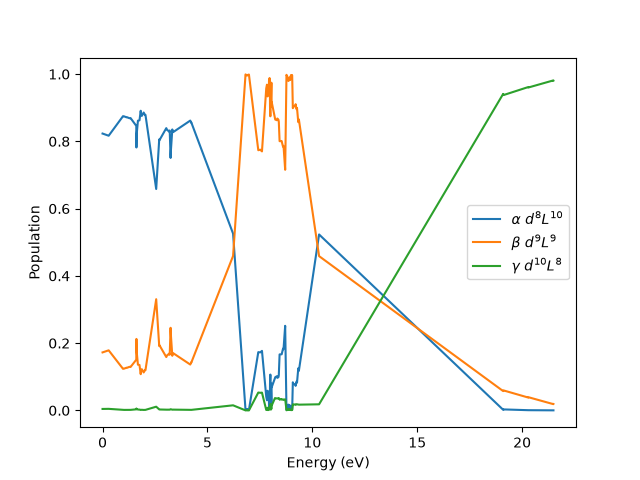
This example follows the Anderson impurity model for NiO XAS example and considers the same model. This time we show how to analyze the eigenvectors in terms of a \(\alpha |d^8L^{10}\rangle + \beta |d^9L^9\rangle + \gamma |d^{10}L^8\rangle\) representation.

Hamiltonian

We start by obtaining all eigenvectors of the previous Hamiltonian.

import numpy as np
import matplotlib.pyplot as plt
import edrixs

backend = 'scipy'
eval_i, evec_i = edrixs.ed(hmat_i, shift=shift, num_evals=len(basis_i), backend=backend)
eval_i = eval_i - eval_i.min()

/home/runner/micromamba/envs/build-env/lib/python3.12/site-packages/edrixs/scipy_backend/scipy_backend.py:98: UserWarning: The problem size 190 minus the constraints size 0 is too small relative to the block size 190. Using a dense eigensolver instead of LOBPCG iterations.No output of the history of the iterations.
  eigenvalues, eigenvectors = lobpcg(

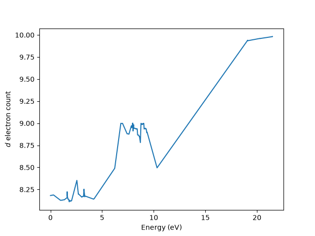
Number of d electrons

We can count the number of \(d\) electrons by building a single-particle operator single_particle_Nd with ones on the diagonal at the nickel \(d\)-shell orbitals and zeros elsewhere. build_op() transforms this into the many-body operator O, whose expectation value in each eigenvector is the \(d\)-electron count of that state.

single_particle_Nd = np.zeros_like(emat_i)
single_particle_Nd[:norb_d, :norb_d] = np.eye(norb_d)

O = edrixs.build_op(single_particle_Nd, None, basis_i, backend=backend)

nd_expect = np.sum(evec_i.conj() * (O @ evec_i), axis=0).real

fig, ax = plt.subplots()

ax.set_xlabel('Energy (eV)')
ax.set_ylabel('$d$ electron count')
ax.plot(eval_i, nd_expect)

[<matplotlib.lines.Line2D object at 0x7f65479c22d0>]

Configuration weights alpha, beta, gamma

Every Fock state has a definite \(d\) occupation, so \(O\) is diagonal in the Fock basis. O.diagonal() therefore gives the \(d\)-electron count of each Fock-basis component, in the same order as the amplitudes of the eigenvectors returned by ed().

nd_per_component = np.rint(O.diagonal().real).astype(int)

amp2 = np.abs(evec_i)**2
alphas = amp2[nd_per_component == 8].sum(axis=0)
betas = amp2[nd_per_component == 9].sum(axis=0)
gammas = amp2[nd_per_component == 10].sum(axis=0)

print("Ground state\nalpha={:.3f}\tbeta={:.3f}\tgamma={:.3f}".format(
    alphas[0], betas[0], gammas[0]))

fig, ax = plt.subplots()
ax.plot(eval_i, alphas, label=r'$\alpha$ $d^8L^{10}$')
ax.plot(eval_i, betas, label=r'$\beta$ $d^9L^{9}$')
ax.plot(eval_i, gammas, label=r'$\gamma$ $d^{10}L^{8}$')
ax.set_xlabel('Energy (eV)')
ax.set_ylabel('Population')
ax.legend()

Ground state
alpha=0.823     beta=0.172      gamma=0.004

<matplotlib.legend.Legend object at 0x7f654739ffb0>