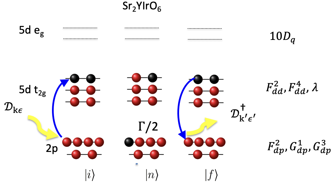
RIXS calculations for an atomic model#
Here we show how to compute RIXS for Sr₂YIrO₆ based on Ref. [1].
Imports#
import edrixs
import numpy as np
import matplotlib.pyplot as plt

%matplotlib inline
Specify active core and valence orbitals#
shell_name = ('t2g', 'p32')
v_noccu = 4
Slater parameters#
The paper specifies the valence Coulomb interactions and spin orbit coupling [1][2]. Other interaction parameters can be loaded from a database containing Hartree-Fock predictions.
F2_dd = 2.15
F4_dd = 1.34
lam = 0.42

info = edrixs.utils.get_atom_data('Ir', '5d', v_noccu, edge='L3')
G1_dp = info['slater_n'][5][1]
G3_dp = info['slater_n'][6][1]
F2_dp = info['slater_n'][4][1]

slater = [[0, F2_dd, F4_dd],
          [0, F2_dd, F4_dd, 0, F2_dp, G1_dp, G3_dp]]
v_soc = (lam, lam)
Diagonalization#
Since we have already specified a \(t_{2g}\) subshell only, we do not need to pass an additional v_cfmat matrix.
Note that we need to tune the energy of the intermediate state via off.
off = 11216
out = edrixs.ed_1v1c_py(shell_name, shell_level=(0, -off), v_soc=v_soc,
                        c_soc=info['c_soc'], v_noccu=v_noccu, slater=slater)
eval_i, eval_n, trans_op = out
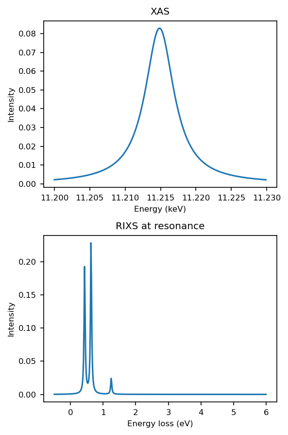
Compute XAS#
ominc = np.arange(11200, 11230, 0.1)
temperature = 300  # in K

thin = np.deg2rad(30)
pol_type = [('linear', 0)]

xas = edrixs.xas_1v1c_py(
    eval_i, eval_n, trans_op, ominc, gamma_c=info['gamma_c'],
    thin=thin, pol_type=pol_type)
The array xas will have shape (len(ominc), len(pol_type)).
Compute RIXS#
eloss = np.linspace(-.5, 6, 400)
pol_type_rixs = [('linear', 0, 'linear', 0), ('linear', 0, 'linear', np.pi/2)]
gs_list = [0, 1, 2]
thout = np.deg2rad(60)
gamma_f = 0.02

rixs = edrixs.rixs_1v1c_py(
    eval_i, eval_n, trans_op, ominc, eloss,
    gamma_c=info['gamma_c'], gamma_f=gamma_f,
    thin=thin, thout=thout,
    pol_type=pol_type_rixs, gs_list=gs_list,
    temperature=temperature
)
The array rixs will have shape (len(ominc), len(eloss), len(pol_type)).
Plot XAS and RIXS#
What do you expect the XAS spectrum to look like?
Why is there zero elastic intensity and what could I alter in the experimental geometry in order to see elastic intensity?
fig, axs = plt.subplots(2, 1, figsize=(4, 6))

def plot_it(axs, ominc, xas, eloss, rixscut, rixsmap=None, label=None):
    axs[0].plot(ominc/1000, xas[:, 0], label=label)
    axs[0].set_xlabel('Energy (keV)')
    axs[0].set_ylabel('Intensity')
    axs[0].set_title('XAS')

    axs[1].plot(eloss, rixscut, label=f"{label}")
    axs[1].set_xlabel('Energy loss (eV)')
    axs[1].set_ylabel('Intensity')
    axs[1].set_title(f'RIXS at resonance')

rixs_pol_sum = rixs.sum(-1)
cut_index = np.argmax(rixs_pol_sum[:, eloss < 2].sum(1))
rixscut = rixs_pol_sum[cut_index]

plot_it(axs.ravel(), ominc, xas, eloss, rixscut, rixsmap=rixs_pol_sum)
plt.tight_layout()
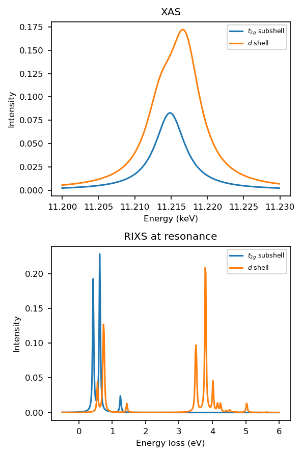
Full d shell calculation#
Does it make sense to consider only the \(t_{2g}\) subshell [3]?
How will the XAS and RIXS spectra change when including the \(e_{g}\) states?
ten_dq = 3.5
v_cfmat = edrixs.cf_cubic_d(ten_dq)


out = edrixs.ed_1v1c_py(('d', 'p32'), shell_level=(0, -off), v_soc=v_soc,
                        v_cfmat=v_cfmat,
                        c_soc=info['c_soc'], v_noccu=v_noccu, slater=slater)
eval_i, eval_n, trans_op = out
xas_full_d_shell = edrixs.xas_1v1c_py(
    eval_i, eval_n, trans_op, ominc, gamma_c=info['gamma_c'],
    thin=thin, pol_type=pol_type,
    gs_list=gs_list)
rixs_full_d_shell = edrixs.rixs_1v1c_py(
    eval_i, eval_n, trans_op, np.array([11215]), eloss,
    gamma_c=info['gamma_c'], gamma_f=gamma_f,
    thin=thin, thout=thout,
    pol_type=pol_type_rixs,
    temperature=temperature)
fig, axs = plt.subplots(2, 1, figsize=(4, 6))

plot_it(axs, ominc, xas, eloss, rixscut, label='$t_{2g}$ subshell')
rixscut_d_shell = rixs_full_d_shell.sum((0, -1))
plot_it(axs, ominc, xas_full_d_shell, eloss, rixscut_d_shell, label='$d$ shell')

for ax in axs:
    ax.legend(fontsize=6)
plt.tight_layout()