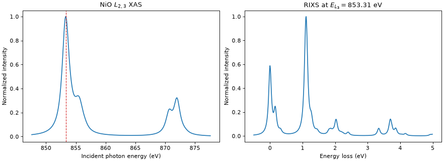
NiO crystal-field \(L_{2,3}\) XAS & RIXS
The calculation treats NiO as an ionic Ni \(3d^8\) site in a cubic field and excites a \(2p\) electron into the \(3d\). It includes an effective exchange field acting along the \(<112>\) direction.
The RIXS spectrum is calculated at the global maximum of the XAS and summed over two orthogonal outgoing linear polarizations.
"""Calculate NiO crystal-field L2,3-edge XAS and RIXS spectra."""

import matplotlib.pyplot as plt
import numpy as np

import edrixs


# Slater integrals
F2_dd, F4_dd = 11.142, 6.874
F2_dp, G1_dp, G3_dp = 6.667, 4.922, 2.796
F0_dd = 2 * (F2_dd + F4_dd) / 63
F0_dp = G1_dp / 15 + 3 * G3_dp / 70

slater_i = [F0_dd, F2_dd, F4_dd]
slater_n = [
    F0_dd, F2_dd, F4_dd,
    F0_dp, F2_dp, G1_dp, G3_dp,
    0.0, 0.0,
]

# emat terms on the 3d shell.
ten_dq = 1.1
zeta_3d, zeta_2p = 0.081, 11.498
exchange = 6 * 0.027
ext_B = exchange / (2 * np.sqrt(6)) * np.array([1.0, 1.0, 2.0])

edge_shift = 857.6
*problem, shift = edrixs.model_1v1c(
    ('d', 'p'),
    shell_level=(0.0, -edge_shift),
    v_soc=(zeta_3d, zeta_3d),
    c_soc=zeta_2p,
    v_noccu=8,
    slater=(slater_i, slater_n),
    v_cfmat=edrixs.cf_cubic_d(ten_dq),
    ext_B=ext_B,
    on_which='spin',
    sparse_U=True,
)

backend = 'scipy'
hmat_i, hmat_n, trans_ops = edrixs.get_ops(*problem, backend=backend)
eval_i, evec_i = edrixs.ed(
    hmat_i, shift=shift,
    num_evals=3,

)

# Calculate XAS spectrum.
energy = np.linspace(edge_shift - 10, edge_shift + 20, 3001)
gamma_c = 0.65
xas = edrixs.xas(
    eval_i, evec_i, hmat_n, trans_ops, energy,
    gamma_c=gamma_c,
    pol_type=[('linear', 0)],

).sum(-1)
xas /= xas.max()

# Calculate RIXS at the global XAS maximum. Summing two orthogonal
# scattered polarizations represents a measurement without outgoing
# polarization analysis.
resonance_energy = energy[np.argmax(xas)]
energy_loss = np.arange(-0.5, 5, 0.01)
rixs = edrixs.rixs(
    eval_i, evec_i, hmat_i, hmat_n, trans_ops,
    np.array([resonance_energy]), energy_loss,
    gamma_c=gamma_c,
    gamma_f=0.05,
    pol_type=[
        ('linear', 0, 'linear', 0),
        ('linear', 0, 'linear', np.pi / 2),
    ],

)
rixs_spectrum = rixs[0].sum(axis=-1)
rixs_spectrum /= rixs_spectrum.max()

fig, (ax_xas, ax_rixs) = plt.subplots(
    1, 2, figsize=(11, 4), constrained_layout=True
)
ax_xas.plot(energy, xas)
ax_xas.axvline(resonance_energy, color='tab:red', linestyle='--', linewidth=1)
ax_xas.set_xlabel('Incident photon energy (eV)')
ax_xas.set_ylabel('Normalized intensity')
ax_xas.set_title(r'NiO $L_{2,3}$ XAS')

ax_rixs.plot(energy_loss, rixs_spectrum)
ax_rixs.set_xlabel('Energy loss (eV)')
ax_rixs.set_ylabel('Normalized intensity')
ax_rixs.set_title(r'RIXS at $E_{L_3}=%.2f$ eV' % resonance_energy)
plt.show()